The Mathematical Backbone of Modern Solvers for MDO
Understanding Fixed-Point Iteration Methods
In Multidisciplinary Design Optimization, optimizing highly coupled systems requires specialised solvers like Nonlinear Block Jacobi or Nonlinear Block Gauss-Seidel. These advanced algorithms can be difficult to understand without grasping their foundational concept: the fixed-point iteration method.
Despite its simplicity, fixed-point iteration underpins many modern solvers used in numerical analysis to solve linear and nonlinear systems of equations. In this third instalment of the Algorithm Deep Dive series, we’ll explore how fixed-point iteration works and why it’s essential for modern optimization methods.
Curious about other algorithms? Check out our previous articles in this series:
- Genetic Algorithm — From Theory to Practical Implementation
- Newton’s Method — The Powerhouse Behind the Most Efficient Gradient-Based Optimization Algorithms
The Basics of Fixed-Point Iteration: A Simple Example
Suppose you want to solve the following equation:
![]()
The solution is the value of ![]() that satisfies the equation. However, this equation doesn’t lend itself to straightforward manipulation for a direct solution. A more natural and instinctive approach is to test different values for
that satisfies the equation. However, this equation doesn’t lend itself to straightforward manipulation for a direct solution. A more natural and instinctive approach is to test different values for ![]() . For example, substituting
. For example, substituting ![]() gives
gives ![]() , but that’s clearly not the solution.
, but that’s clearly not the solution.
What about ![]() ? Substituting it yields
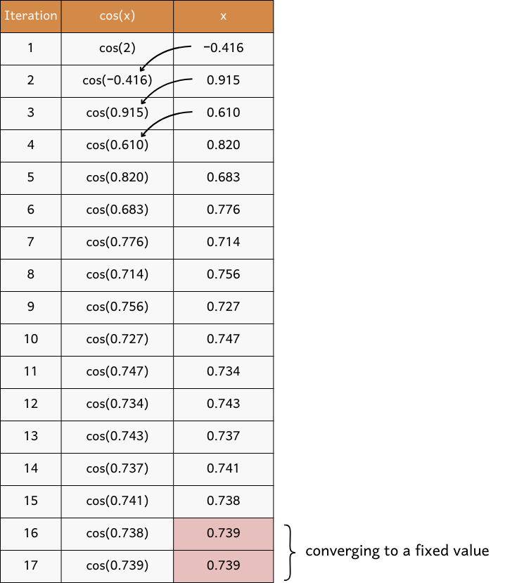
? Substituting it yields ![]() . We’re still not there, but upon repeating the process for a few more times, we see that the result can actually lead to the solution! Precisely, after 16 iterations, the value of
. We’re still not there, but upon repeating the process for a few more times, we see that the result can actually lead to the solution! Precisely, after 16 iterations, the value of ![]() settles at around
settles at around ![]() , satisfying the equation
, satisfying the equation ![]()

 , created by author using Canva
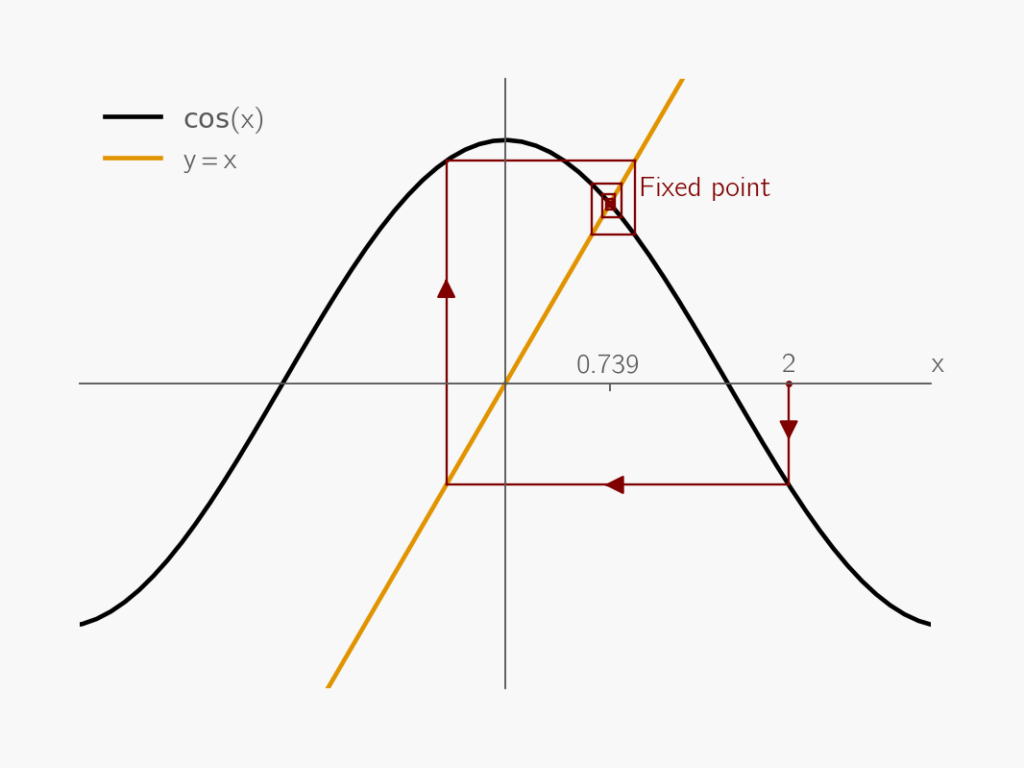
The value ![]() is known as a fixed point of the cosine function. Conceptually, we can visualise the function alongside the line
is known as a fixed point of the cosine function. Conceptually, we can visualise the function alongside the line ![]() . The process of iteratively updating
. The process of iteratively updating ![]() can be represented by the cobweb-like trajectory, where we begin from
can be represented by the cobweb-like trajectory, where we begin from ![]() and converge to the solution at
and converge to the solution at ![]() .
.

Solving Systems of Equations with Fixed Point Iteration
The previous example demonstrates how fixed-point iteration works in a simple case. But how can we generalise this to solve systems of equations? The key is to rearrange the function into the form ![]() , where we can substitute
, where we can substitute ![]() into the function
into the function ![]() in order to get an update in
in order to get an update in ![]() and repeat the process again.
and repeat the process again.
For linear systems, this target form is often written as:
![]()
Here, ![]() represents the vector of variables, and
represents the vector of variables, and ![]() is a function derived from the system matrix. The subscripts
is a function derived from the system matrix. The subscripts ![]() and
and ![]() represent the current and next iterations respectively.
represent the current and next iterations respectively.
In this section, we’ll introduce two methods, Jacobi and Gauss-Seidel, which utilise the fixed-point iteration concept by reformulating a linear system into the above target form to solve it efficiently.
The Jacobi Algorithm
Given the general form of a linear system of equations:
![]()
Where ![]() and
and ![]() are matrix and vector of some known values respectively, and
are matrix and vector of some known values respectively, and ![]() is the vector of variables that we are trying to solve for.
is the vector of variables that we are trying to solve for.
The Jacobi algorithm works by splitting ![]() into a diagonal matrix
into a diagonal matrix ![]() and a matrix
and a matrix ![]() with zeros on the diagonal:
with zeros on the diagonal:

Substituting into ![]() and rearranging gives:
and rearranging gives:
![]()
Since ![]() is a diagonal matrix, its inverse is easy to compute. The Jacobi method updates
is a diagonal matrix, its inverse is easy to compute. The Jacobi method updates ![]() iteratively by calculating the new
iteratively by calculating the new ![]() based on the previous
based on the previous ![]() , following the fixed-iteration framework.
, following the fixed-iteration framework.
The Gauss-Seidel Algorithm
The Gauss-Seidel algorithm takes a slightly different approach. Instead of splitting ![]() into a diagonal matrix, it splits
into a diagonal matrix, it splits ![]() into upper and lower triangular matrices
into upper and lower triangular matrices ![]() and
and ![]() :
:

This gives the iteration form:
![]()
Unlike Jacobi, Gauss-Seidel updates the variables one at a time, using the most recent values of the other variables as soon as they become available, which typically results in faster convergence.
Some Notes on Convergence
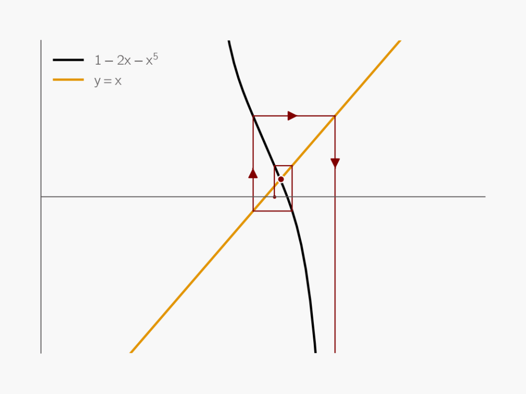
In the case of ![]() , the fixed point is attracting, meaning nearby starting points converge toward the solution. However, not all fixed points are attracting. For instance, the fixed point in the function
, the fixed point is attracting, meaning nearby starting points converge toward the solution. However, not all fixed points are attracting. For instance, the fixed point in the function ![]() can repel, causing divergence during iteration.
can repel, causing divergence during iteration.

 , created by author using matplotlib
For linear systems, convergence is guaranteed if the matrix ![]() is diagonally dominant, meaning the magnitude of the diagonal elements is larger than the off-diagonal elements in the same row. Pivoting, which reorders rows or columns to achieve diagonal dominance, can help ensure convergence and is often built into numerical solvers.
is diagonally dominant, meaning the magnitude of the diagonal elements is larger than the off-diagonal elements in the same row. Pivoting, which reorders rows or columns to achieve diagonal dominance, can help ensure convergence and is often built into numerical solvers.
For nonlinear systems, convergence is less predictable. Factors such as the system’s nonlinearity, coupling strength, and initial guess play significant roles. Techniques like relaxation or under-relaxation can sometimes improve convergence in difficult cases.
Conclusions
Fixed-point iteration is a foundational concept in numerical solvers, especially for Multidisciplinary Design Optimization. Although the process may appear mindless, it eventually works given the right conditions of an attracting fixed point.
This method offers several key benefits, the most notable one being its simplicity. Fixed-point iteration transforms complex equations into a straightforward iterative process that can be applied repeatedly until convergence is achieved. Unlike direct solvers, which provide an exact solution only at the end, fixed-point iteration allows users to monitor progress and trade between computational cost and precision as needed.
In this article, we explored two key fixed-point algorithms — Jacobi and Gauss-Seidel. While both follow a similar iterative procedure, Gauss-Seidel generally offers faster convergence due to its update strategy.
Understanding these solvers is crucial in optimization tasks, helping engineers recognise limitations, improve performance, and diagnose irregularities. I hope this deep dive has been useful!
If you have suggestions for other algorithms you’d like to see covered, feel free to leave a comment!
At OptimiSE Academy, we’re excited to announce our upcoming microcourse on Optimization Mathematics. This course provides an intuitive foundation for design optimization. Sign up for the waitlist here!

Leave a Reply